Random Variables, and the CDF

Beginning of Chapter Three

Random Variables

• Map events to numbers so that we can use math.
• If we have a random variable, it must be a capital letter (X)
• A lower case letter (x) is known as a realization. I,e numbers we know

Example 1

Let X_i = 1 is an apple is picked from a barrel on the ith pick, and X_i = 0 if an orange is picked from a barrel.

$$\sum _{i=1}^n{x}_i=(0+1+1+0+\mathrm{0...})=17\text{(For}\text{Example)}$$

This means that we picked 17 apples, and if we picked n total items, we picked n - 17 oranges.

Example 2

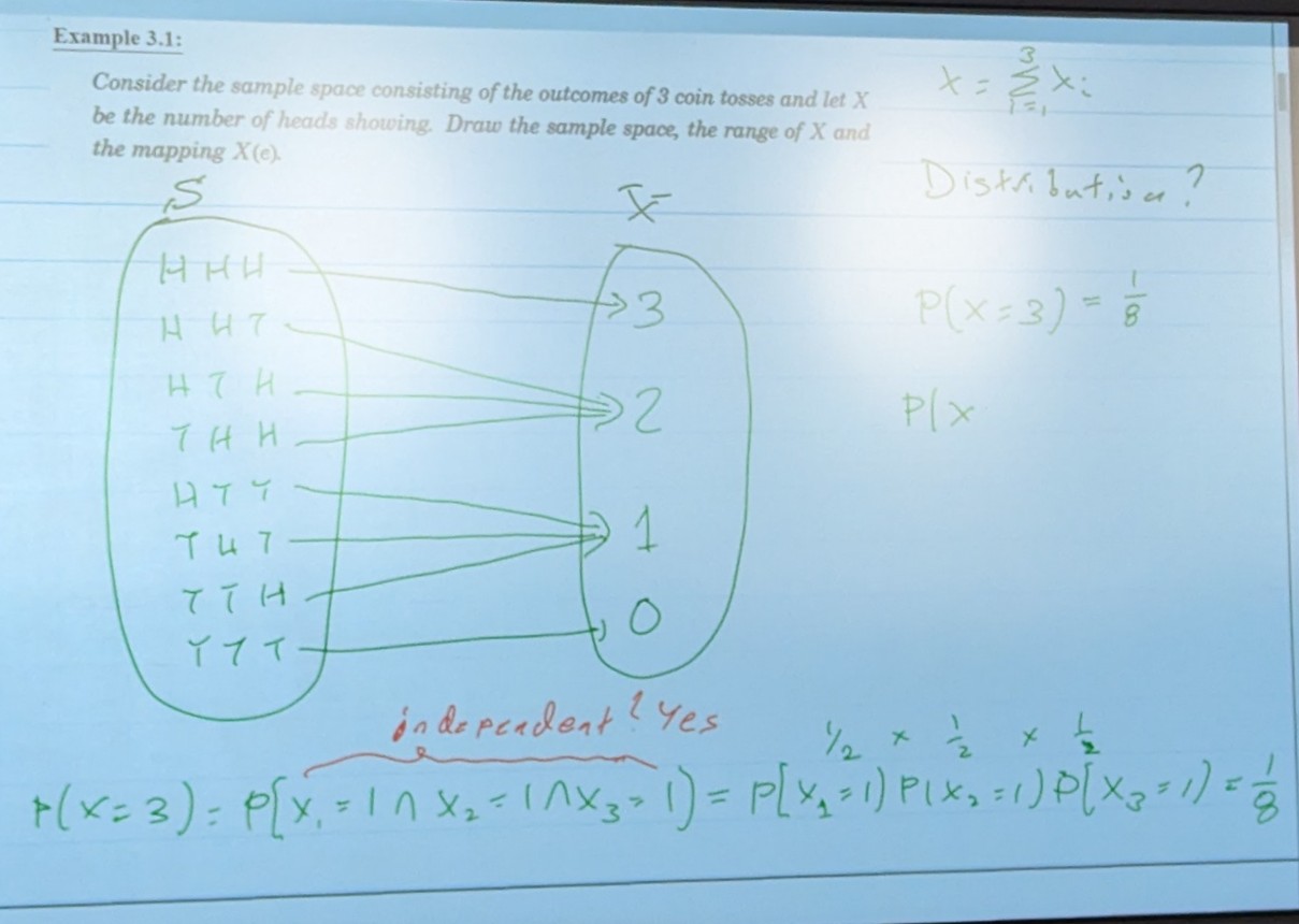
Be sure to remember to check for independence and disjointedness for unions and overlaps!

---

• The most we can say about X (the random variable) is what its probability is of taking on any of its possible values.

• This is called a Probability Distribution

Cumulative Distribution Function (CDF)

Definition:

$$F_x(x)=P(X\leqq x)$$

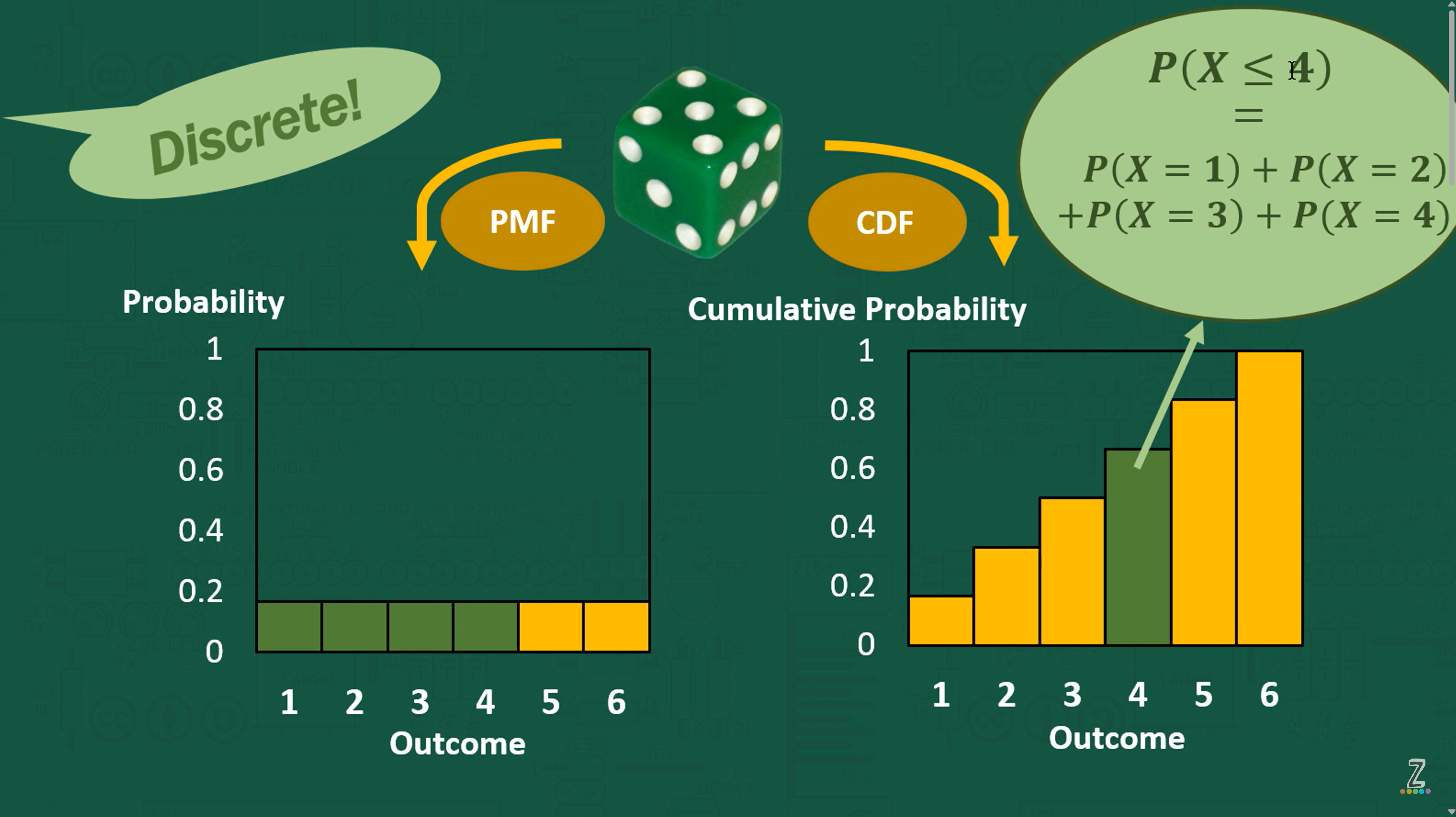
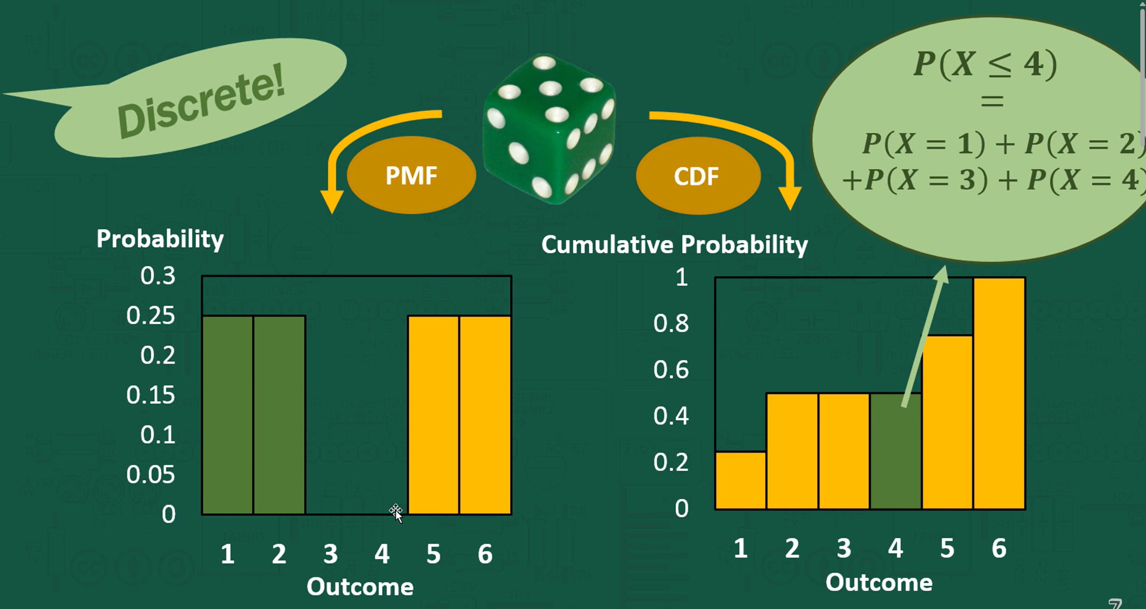
• If there is no “mass” at a certain number, it will affect the CDF accordingly.

In the previous example 3.1, the CDF is

$$F_x(-1)=P(X\leqq -1)=0$$ $$F_x(0)=P(X\leqq 0)=\frac{1}{8}$$ $$F_x(0.5)=P(X\leqq 0.5)=\frac{1}{8}$$ $$F_x(1)=P(X\leqq 1)=\frac{1}{8}+\frac{3}{8}=\frac{1}{2}$$

(Here, it is the previous chances summed)

$$F_x(2)=P(X\leqq 2)=\frac{1}{8}+\frac{3}{8}+\frac{3}{8}=\frac{7}{8}$$ $$F_x(2)=P(X\leqq 3)=1$$

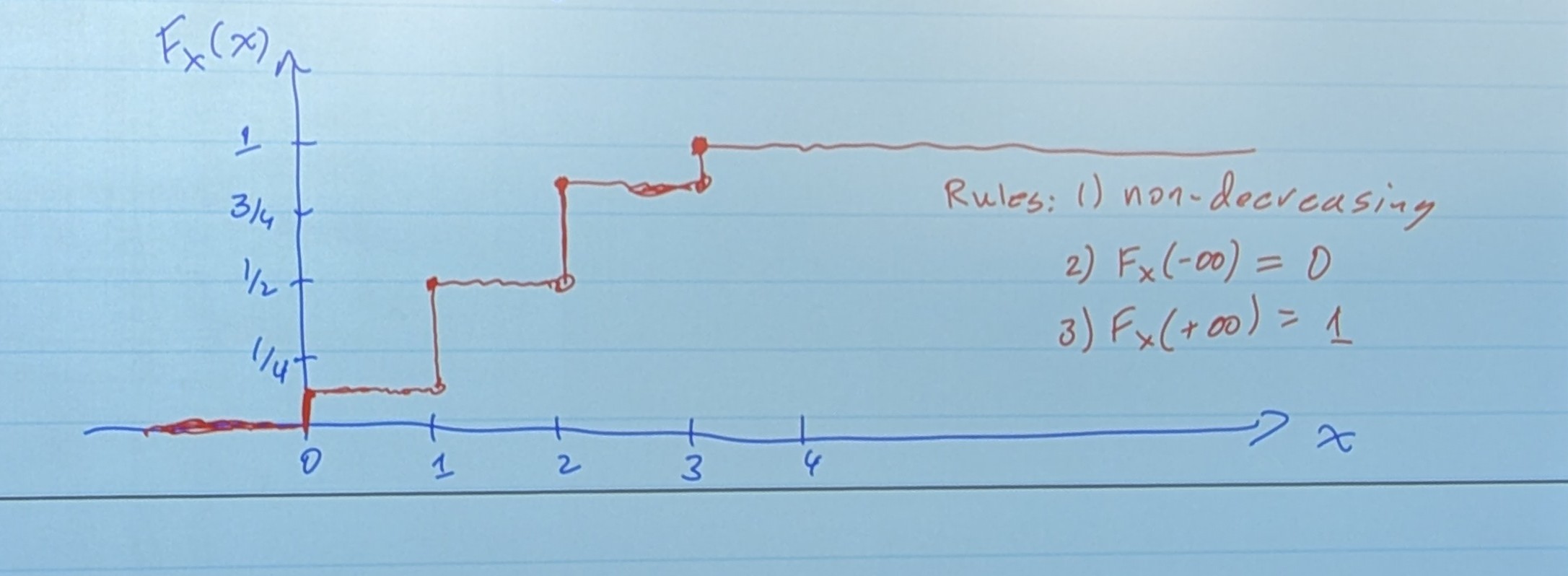
This accumulates distributions.

So you also see the rules of these CDF’s listed above!

1. CDF’s are non-decreasing. They only grow.
2. $F_x(-\infty )=0$
3. $F_x(\infty )=1$
4. The final bar has to be one! The CDF has to be one at the end.

So, you may be asking… How do we get P(X=x) if you know F_x (x)

$$P(X=1)=F_x(2)-F_x(1)$$

So we can construct P(X=x) given F_x (x) and vice versa

We can say that these are equivilent.

---

Types of Random Variables

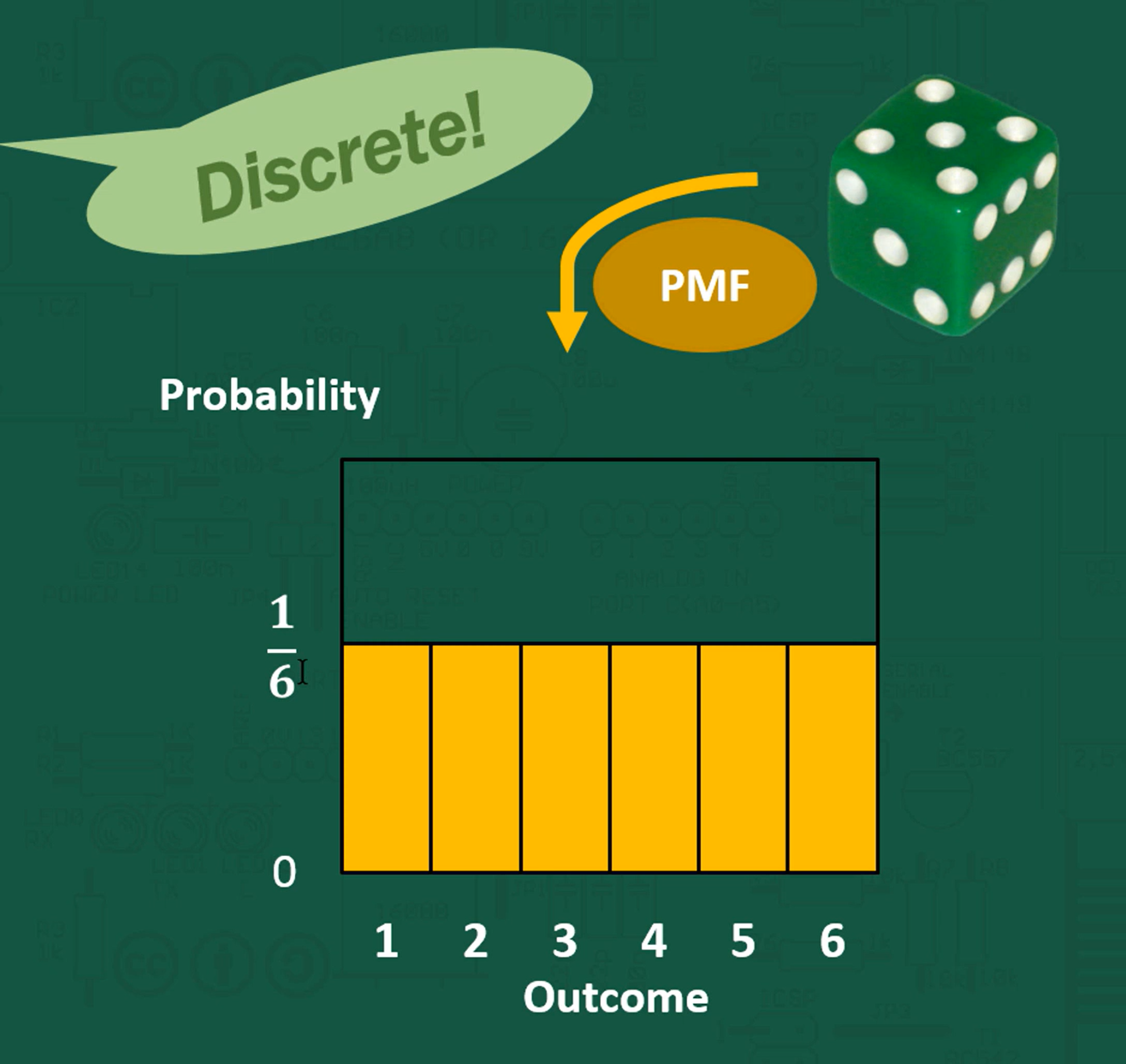
1. Discrete:
   • X takes on a countable number of possible values
   • Examples:
     1. 3 - coin toss
     2. A deck of cards
     3. Temperature (if rounded)
     4. Number of students in a class

Note

These are defined by a probability mass function (pmf).

$$P(X=x_1),P(X=x_2),...,P(X=x_n)$$

2. Continuous Random Variables
   • X takes on a uncountable number of possible outcomes

Example

Sample Space: S = all real numbers from 0 to infinity

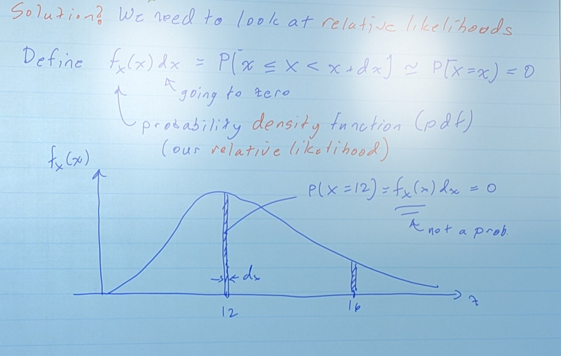
Distribution?

$$P(T=\mathrm{12.000000000000000.........000})=0$$ $$P(T=\mathrm{12.100000000000000.........000})=0$$

All P(X = x) =0

• The curve here is helping us represent the chance of failure at a time. A taller area at a time, with your little slice of dx, shows that at 12, the probability of failure is MUCH higher than at 16. This is what the probability density function is useful for.

• We are multiplying this “density function”, by volume (in 1d in this case) to get back to the mass function.

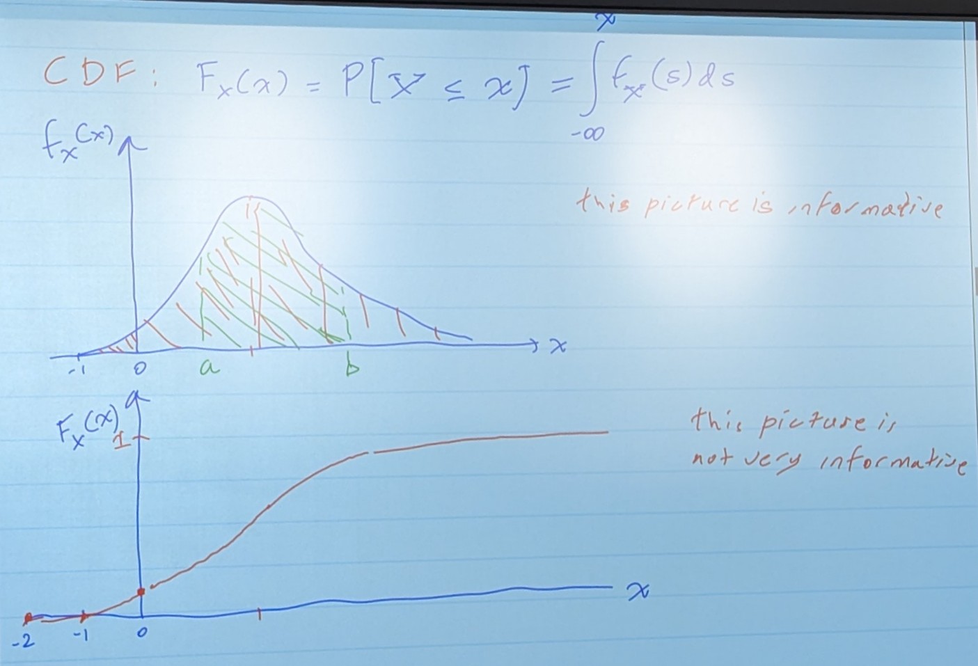
Usually, we look for these probabilities in terms of ranges

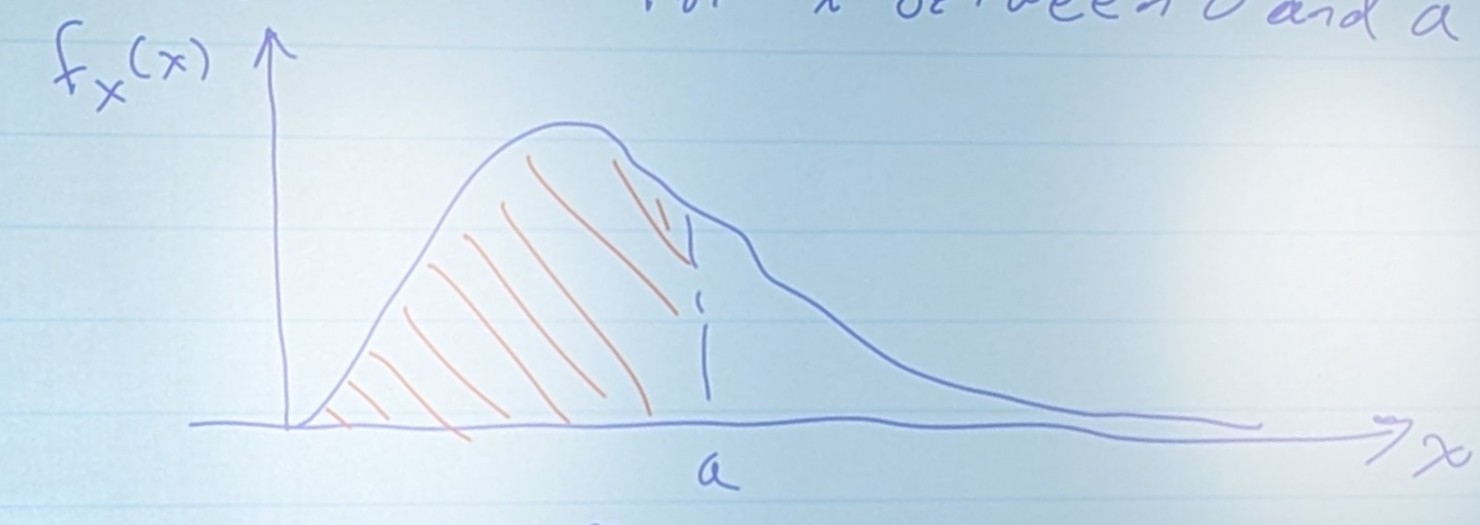
And you’ll never guess how we sum all the little parts under the curve!

$${\int }_0^a(P(X=x))$$ $${\int }_0^a(F_X(x)dx$$

So, for something like P(X ⇐ a) would be

$${\int }_{-\infty }^a(F_X(x)dx$$

Something like P(a < x < b) would be

$${\int }_a^b(F_X(x)dx=Fx(b)-Fx(a)$$

So actually, the integral and CDF are the same thing! The CDF is just a solved integral

In terms of CDF

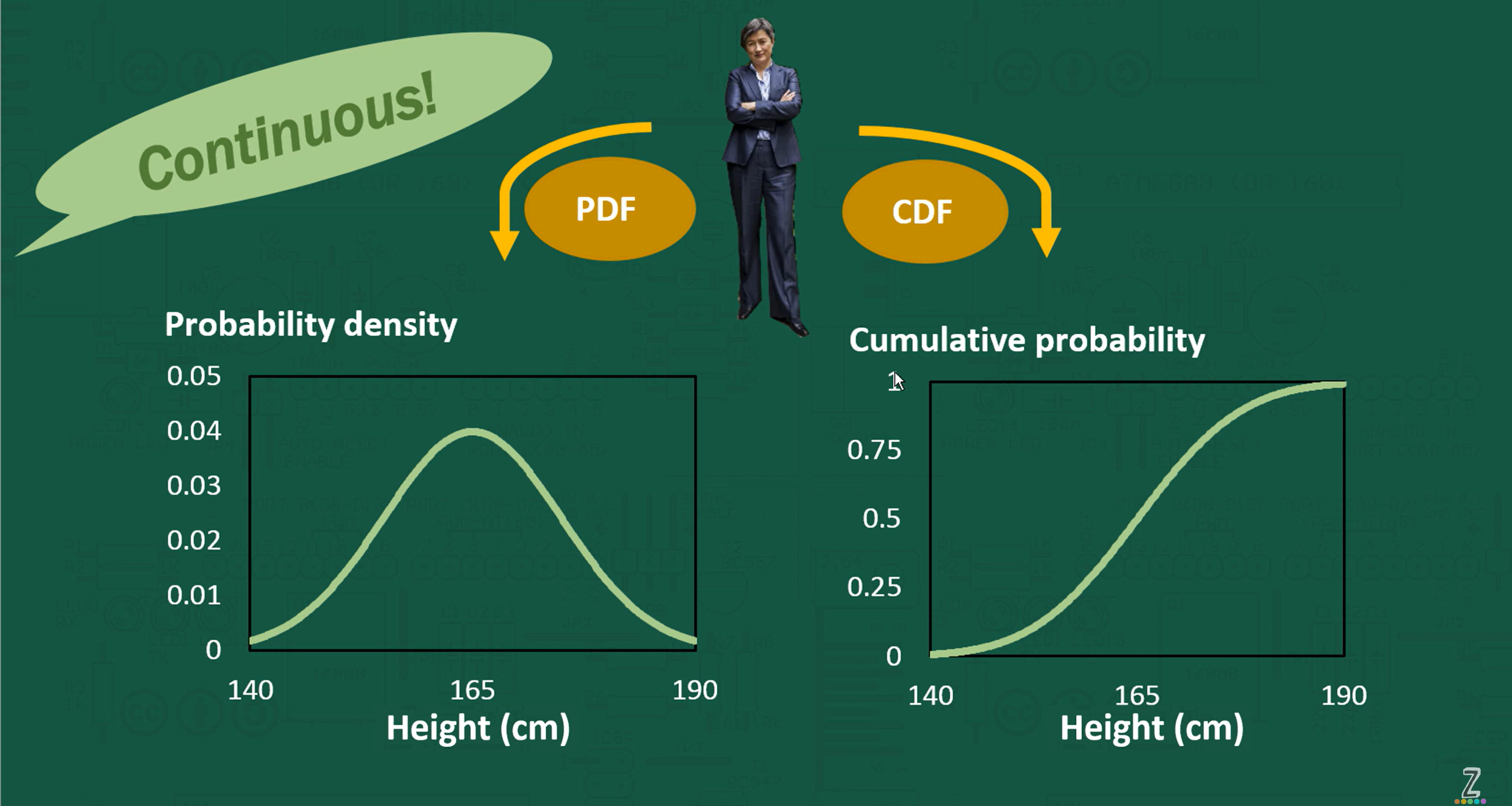
PDF = fx (The integral, nicer graph, but you have to compute an integral) CDF = Fx (Much easier to solve, but a crappier graph)

Note

These are defined by a probability density function (pdf).

$$f(x)$$

This is denoted by little f(x), and will need to be integrated

• A higher gradient on a CDF, would indicate a period of higher gradient indicating a period of higher density.

Main Descriptors

Central Tendency:

• Mean: μx = balance point of the pdf = Centroid of the area

= Sum of all possible values times their probability of occurrence.