Polar Coordinates, Cylindrical Systems, Spherical Systems

Polar Coordinates

x = rcosθ y = rsinθ

• Polar Coordinates are another way of representing graph systems
• How to we apply polar coordinates to what we have been doing with double and triple integrals?

$${\iint }_{Rxy}f(x,y)dxdy={\iint }_{Rr\theta }g(r,\theta )rdrd\theta$$

• There is a proof for this, but this is what we feed into our double and triple integrals for polar coordinates!
• You can use polar coordinates for functions that are not nice with regular coordinates.
• A classic example of such would be x² + y² = 1

Polar Coordinates for Double Integrals

Step One: Convert from f(x,y) to g(r, θ)

Step Two: Convert dx/dy to dArθ - Tip for this, it will ALWAYS be rdrdθ

Step Three: Convert limits (Plug in and work out) - This can be a bit tricky.

Step Four: Now, integrate as normal. U-Sub may be needed

---

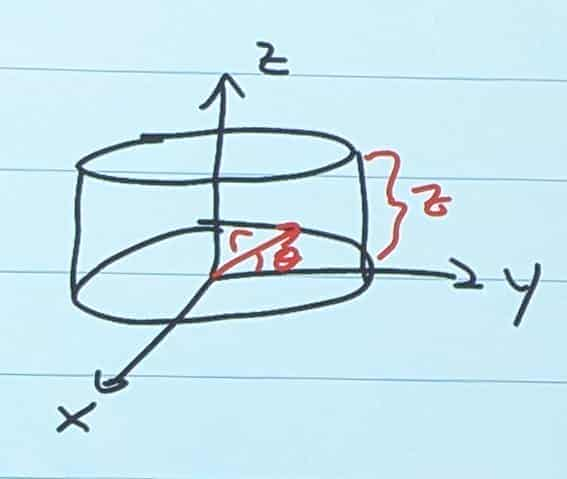
Polar Coordinates for Triple Integrals

Now, we are dealing with cylindrical coordinates! (Polar in 3D)

x = rcosθ y = rsinθ z = z

dVol ⇛ dxdydz ⇛ rdrdθdz

• Volume = ∫∫∫dVol

---

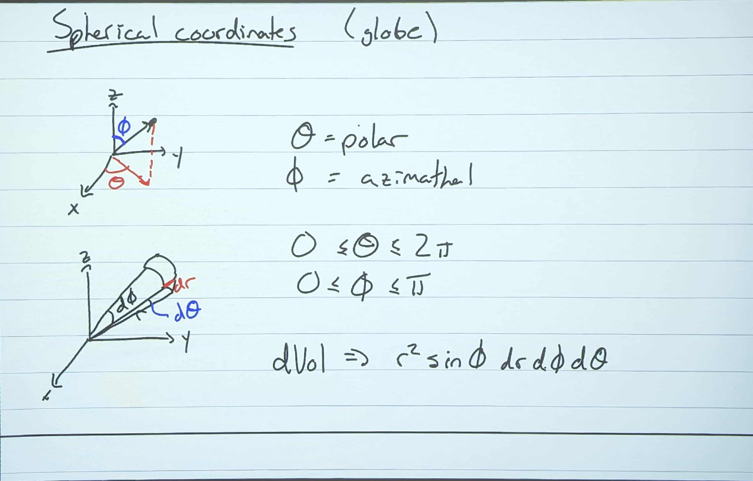
Spherical Coordinates (Globe)

x = rcosθsinϕ y = rsinθsinϕ z = rcosϕ

r² = x² + y² +z²

• With Spherical Coordinates, you are going to have an R like usual
• However, you are going to have TWO angles
• A polar angle along X and Y, and an azimuthal angle along Z
• The regular angle can stretch from 0 < θ < 2π
• The azimuthal angle can stretch from 0 < ϕ < π
  • It is not necessary for the full 2π, as you would be double accounting for each position

• Remember with U-sub, you can either change your limits in terms of U, or sub in for you after the integration with the original limits

---

END OF TEST 2 MATERIAL

Vector Spaces

• A vector spaces is a set of vectors

• Addition and Scalar multiplication can be used!

• Vector spaces can be anything, vectors, polynomials, functions

• If I have two polynomials of the first degree , u = x + 1 and v = 2x - 3, they both share the same vector space, because they are same degree

• If I add the polynomials u = x + 1 and v = 2x - 3 together, I get uv = 3x - 2

• The resulting uv = 3x - 2 is also a polynomial of degree one, so we’re still in that original vector space!

• The same is true if I multiplied u = x + 1 by 5. I would get 5u = 5x +5. 5u is still a polynomial of degree one, so we’re still in that first degree polynomial space!

—

• The same is true of I have the two matrices

$$\hat{u}=\left[\begin{array}{cc}2& 1\\ 1& 3\end{array}\right]$$

and

$$\hat{v}=\left[\begin{array}{cc}-1& 0\\ 1& 1\end{array}\right]$$

• If I add and v̂, I get û + v̂

$$\hat{u}+\hat{v}=\left[\begin{array}{cc}1& 1\\ 2& 4\end{array}\right]$$

• This results in a 2D vector, meaning that we are staying in the same 2D vector space.
• 5û would result in the same thing, another 2D vector. We’re good here.

—

These are known as the properties of closure.

• Given ûεV (û is a vector in the vector space V) and scalar C, then Cûε V (The multiplied scalar will also be in vector space V)

• Given ûεV and v̂εV , then û + v̂ϵ V (The new added vector is also in vector space V!)

The dimension of the vector is usually noted by ℝⁿ. The amount of non zero rows in a vector will give you that.

—

What are Axioms? What are the 8 Axioms?

Axioms are a bunch of rules which hold true inside of a vector space. There are 10 of which hold true in any vector space V

With vectors û, v̂ and ŵ, and scalars a and b

Addition

1. û + v̂ = v̂ + û This is known as the commutative property of addition!

2. û + (v̂ + ŵ) = (û + v̂) + ŵ This is known as the associative property

3. û + 0 = û + 0 There is a zero vector. This is known as the additive identity

4. û + û' For every vector in a vector space, there is another vector that can bring it back to zero. This property is known as the additive inverse! Multiplication

5. For ûϵ**V* 1û = u For every single vector in the vector space V, 1* û will equal û. This is known as the multiplicative identity

6. a * (bu) = (ab) * u This property does not seem to have a name, but is used to combine scalars. Scalars can be combined as such.

7. (a + b)u = au + bu This is known as distributivity of scalar multiplication with respect to field addition. Vectors can distribute like this!

8. a(u+v) = au + av This is known as distributivity of scalar multiplication with respect to vector addition. Just like the last property, this works as well!