Gradients Revisited and Linear Approximations

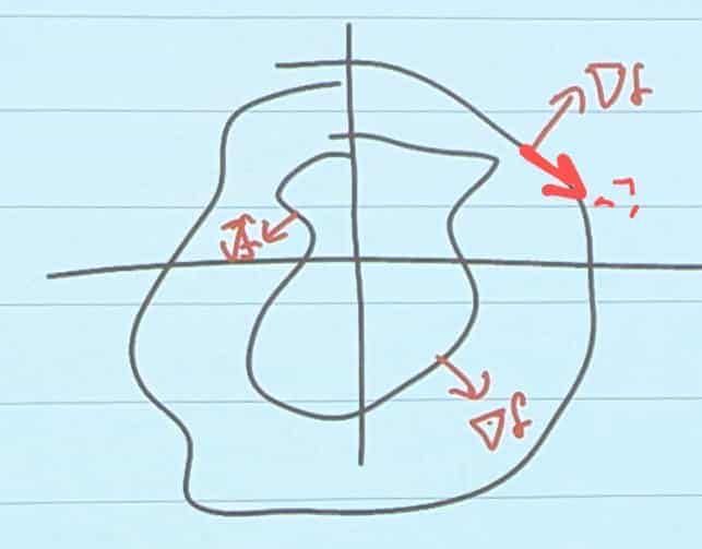
Final Notes about Gradients (Geometric Properties of the gradient)

• As we are moving along a curve in space,∇f is perpendicular to r̂’

---

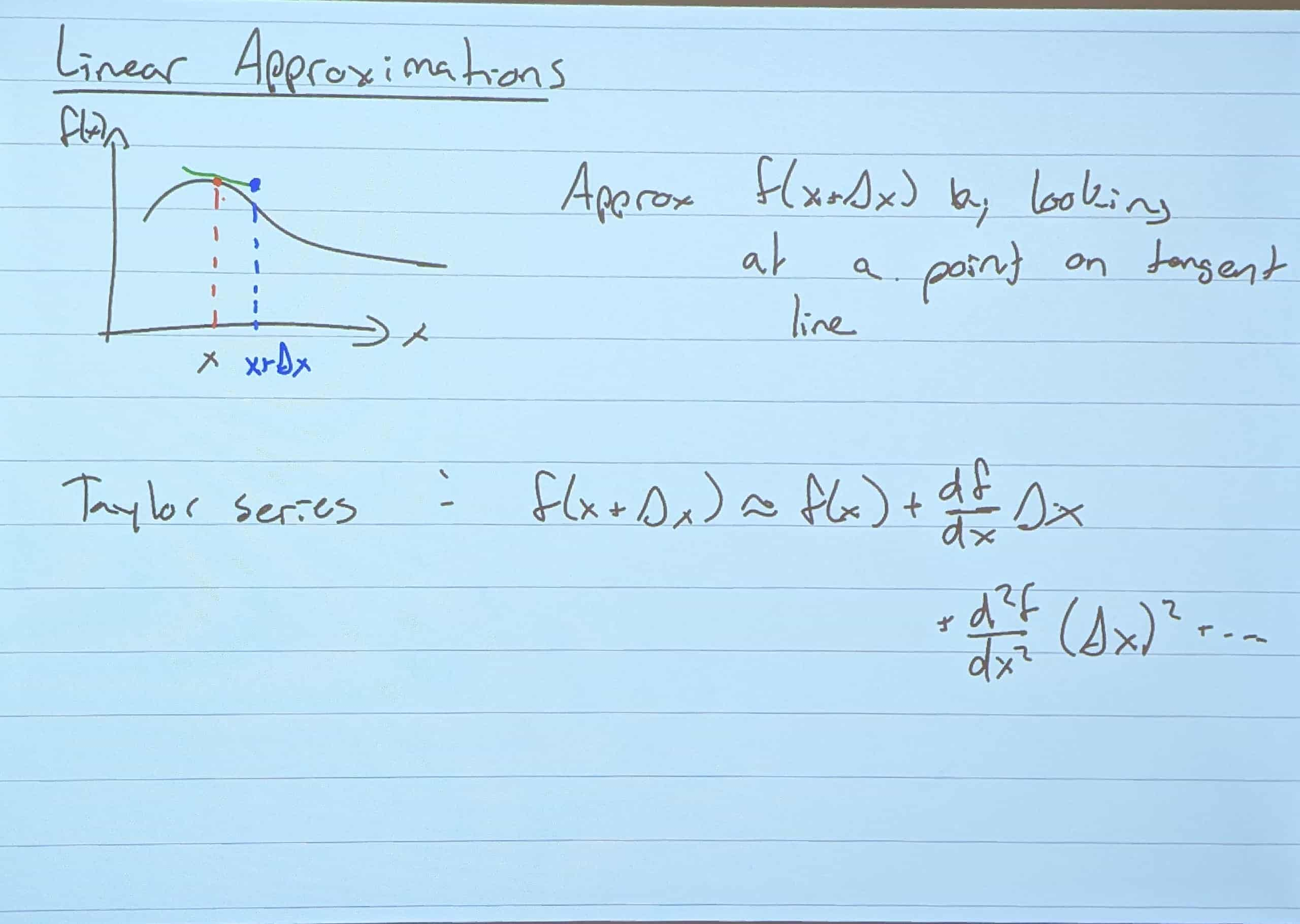
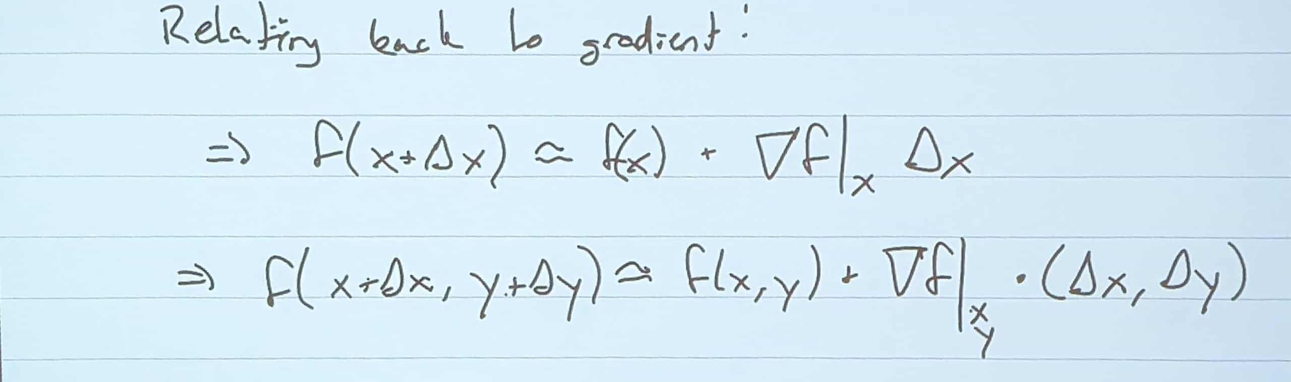
Linear Approximations

• By using the tangent line of an earlier point, we can approximate a later point on a curve
• Maybe that isn’t a great method of approximation… so let’s use higher derivatives to help!
• This is Taylor Series!

• What’s cool, is we can also approximate a “tangent plane” in a similar way!

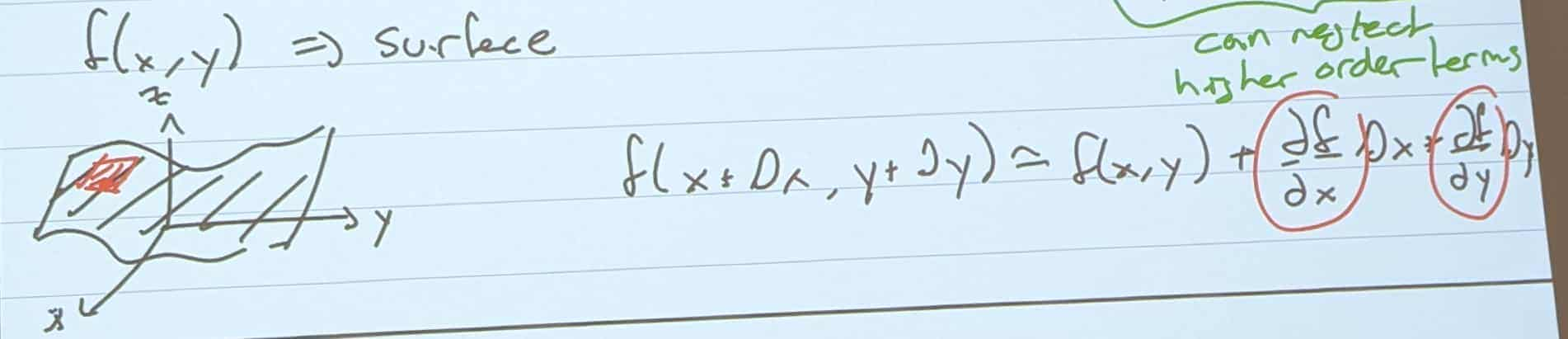
• Usually, a first order approximation is… good enough. More so would be more accurate, but a pain to write out.

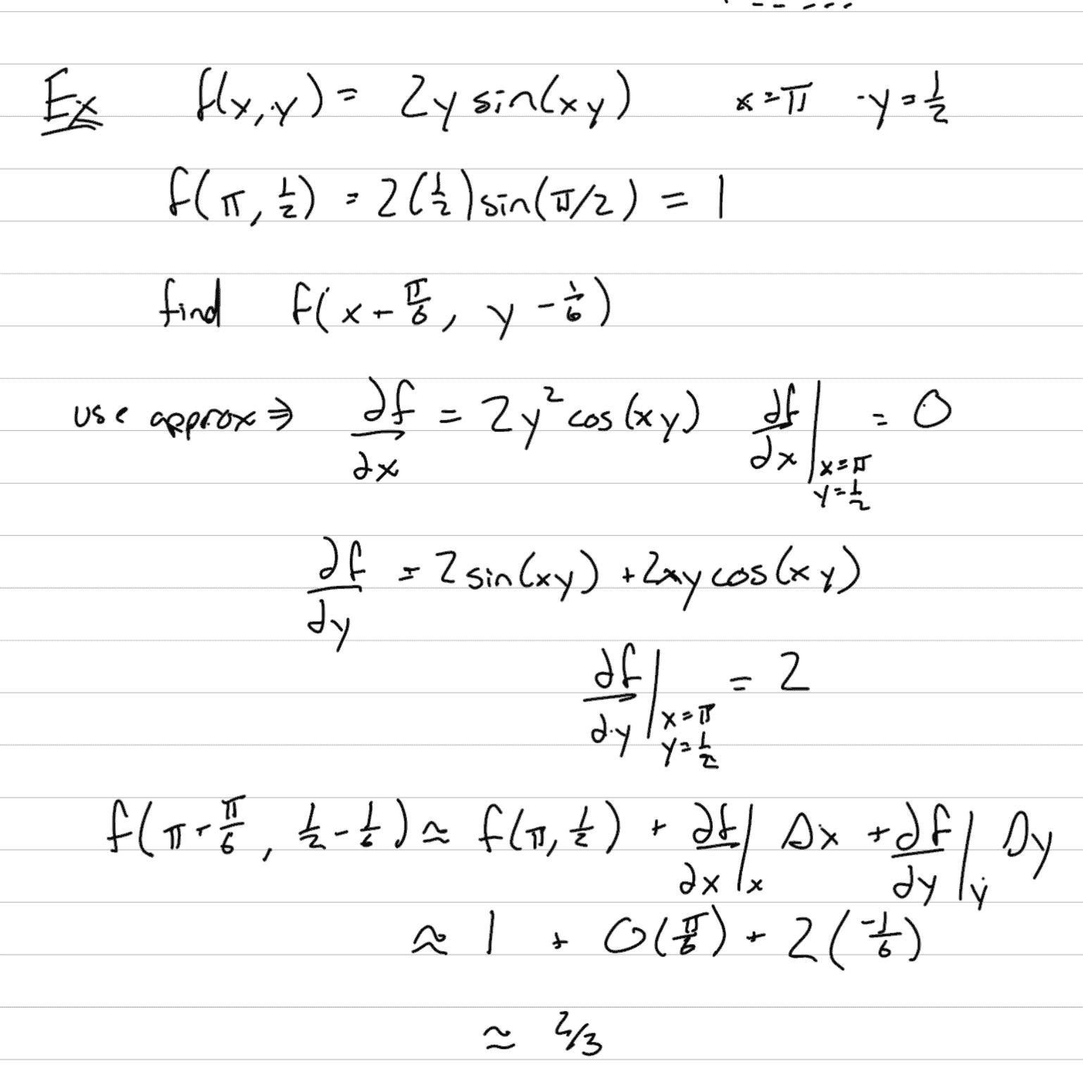
The Gradient is related to linear approximation!

---

Extreme Values (Minimums and Maximums)

For a single variable function y=f(x)…

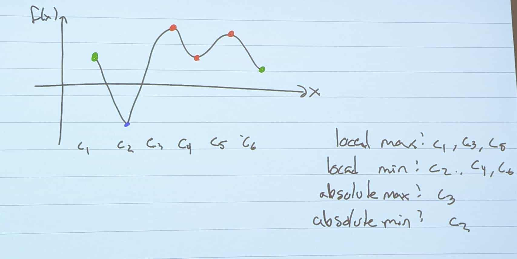
• Extreme Values of Y at x =c If f(x)<f(c) for x near c, you have a local max If f(x)>f(c) for x near c, you have a local min

• Extreme Values occur at 3 types of points

1. Critical Points ⇒ df/dx = 0
2. Singular Points ⇒ df/dx = undefined
3. Boundaries ⇒ The ends

But what if we don’t have a graph?

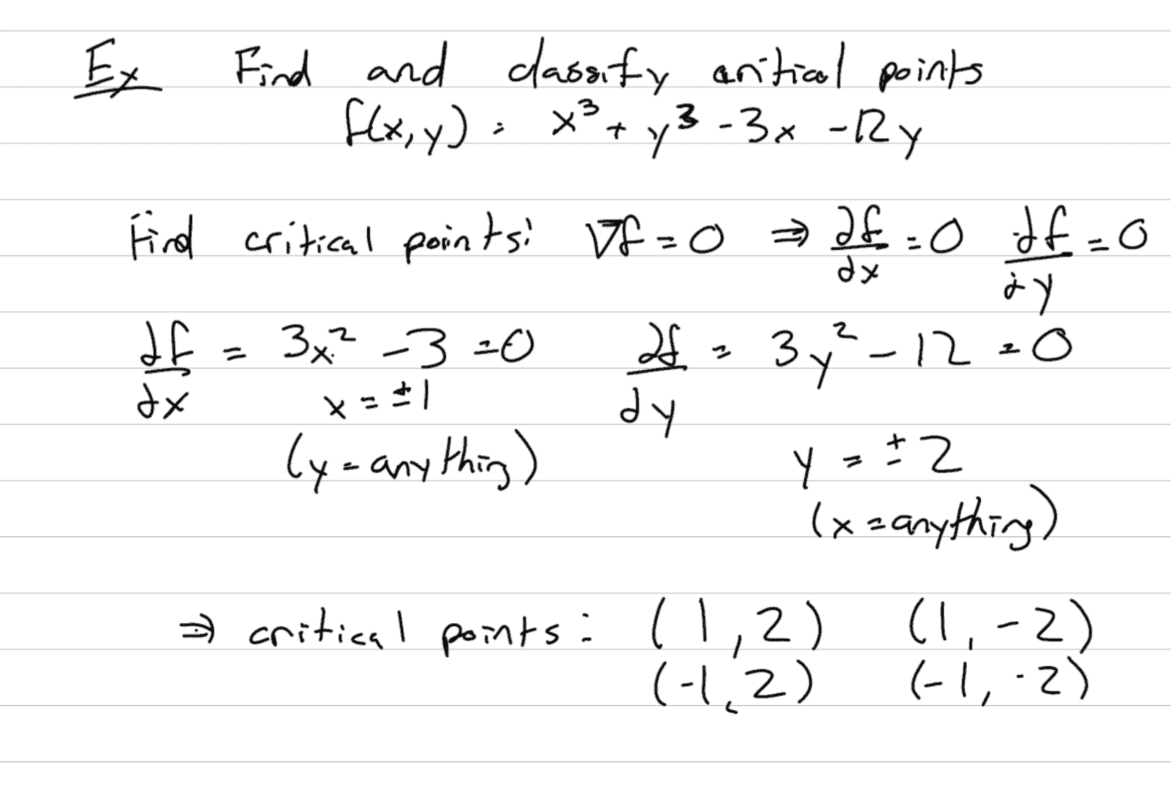
• To find critical points:
  1. Take the first derivative of a function
  2. Set df/dx =0 and solve for X
• To determine minimum or maximum
  1. Take the second derivative of a function. This studies the rate of change of the rate of change
  • If d²f/dx² < 0 ⇒ You have a local max
  • If d²f/dx² > 0 ⇒ You have a local min
  • If d²f/dx² = 0 ⇒ Your curve is flat, and you don’t have enough information!
• If you have a case where d²f/dx² < 0 at some point before the critical point, and where If d²f/dx² > 0 after the critical point, or vice versa, you have an inflection point

For a multivariable function y=f(x,y,z,…)…

Types of Extreme Values

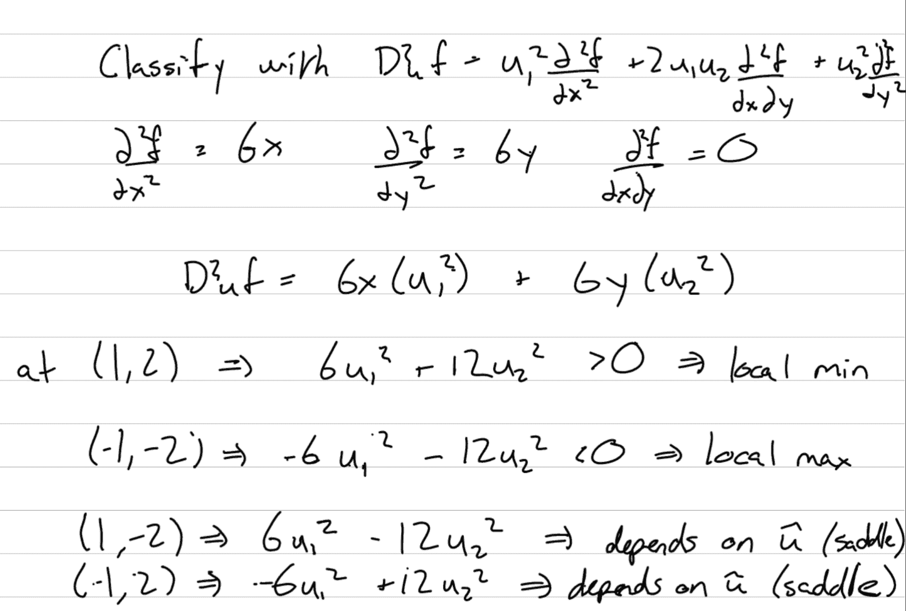
1. Critical Points ⇒ D_uf (The directional derivative) = 0 for all û (for all directions)
2. Singular Points ⇒ D_uf (The directional derivative) = undefined
3. Boundaries ⇒ The ends

$$D_{u}f=\nabla f\cdot \hat{u}$$ $$\text{To have a critical point, }{D}_{u}f\text{ must equal 0}$$ $$\text{If }\nabla f=0,\text{ that makes this true.}$$

Finding critical points: ∇f = 0, solve for points

$$(\frac{\partial f}{\partial x},\frac{\partial f}{\partial y},\frac{\partial f}{\partial z})=(0,0,0)$$

Second Order Directional Derivative! (very bad)

Remember:

• The Gradient nabla operator (∇) vectorizes scalars. That dot product multiplied by the nabla is a scalar, being vectorized. It doesn’t visually mean anything, but makes things

• U_x and U_y are direction vectors

• To determine minimum or maximum

  1. Take the second derivative of a function. This studies the rate of change of the rate of change
  • If d²_uf< 0 for all û (for all directions) ⇒ You have a local max
  • If d²_uf > 0 for all û (for all directions) ⇒ You have a local min
  • If d²_uf< 0 for all û (for all directions) = 0 ⇒ Your curve is flat, and you probably have a saddle point (think the dip in a horse saddle)

Restrictions

• If you are given a restriction, such as x=2, the easiest way to solve the problem is to reduce the dimensionality.

  • Just plug whatever your restriction is into the function, and solve for the other variable’s critical point.